Although I knew about GNU Parallel since a long time, I had never given it a try. I used it recently to launch parametric runs and found it very convenient for single-core simulations. I describe here how I use parallel within a single bash program to control LAMMPS simulations on a HPC node.

What is GNU Parallel and why do I use it for HPC

GNU Parallel is a program from the GNU project (as you can guess from the name). Its purpose is to execute a command several times simultaneously, taking advantage of several cores (or of several machines on a network). You can a series of arguments to parallel to control the execution of the command.

If you have many cores, parallel makes it easy to keep them busy! Even on a laptop it can help to obtain numerical results faster.

A frequent issue I have with running simulations on HPC systems is the need for several files. In addition to the job script that is submitted to the queue and depending on the situation, there can be one parameter file per job or extra scripts. It can become tedious to keep everything in sync. With parallel, I can list several parameters whose permutations will be given to the program.

Simple use of parallel

I first show how to use parallel on a simple test program written in bash:

#!/bin/bash
number=$1
letter=$2
filename=result_${number}_${letter}.txt
echo "letter ${letter}
number ${number}" > $filename

parallel ./myscript.sh ::: 1 2 3 ::: a b c

Parallel will run the program myscript.sh with values 1, 2, and 3 for the first argument of the program and a, b, and c for the second argument. There are two files to manage here: myscript.sh and the job file in which parallel is executed. It is possible to reduce the number of files to one by using a bash function, which I explain in the next section.

Running LAMMPS

Here, I run the LAMMPS simulation program in single-core to show how to perform a parametric run.

parallel ~/path/to/lmp -i in.langevin_1 -var T {1}  ::: 1 2 3

The file is available at in.langevin_1

I have used a single -var argument that sets the variable T in the simulation script (instance of ${T} in in.langevin_1 are replaced by the value of T). This is already very convenient but remains limited.

By using a bash function, it is possible to control more precisely the execution of LAMMPS. I will add a random seed to the program, generated by /dev/urandom. First, I define a seeder function.

generate_seed() { dd count=1 bs=2 if=/dev/urandom 2>/dev/null | od -A n -t u2; }
export -f generate_seed

(Note: it is mandatory to export functions with export -f for them to become available in subprograms.)

Now, I define a function that will process the argument and pass them to LAMMPS, with the random seed, via command line arguments. I also create the output filename in bash as it is more convenient than in LAMMPS.

run_one() {
  T="$1"
  FILENAME=langevin_${T}.dump
  ~/path/to/lmp -i in.langevin_2 -var SEED $(generate_seed) -var T ${T} -var FILENAME ${FILENAME}
}
export -f run_one

The input file is also available in.langevin_2. To run the simulations, I execute

parallel run_one ::: 1 2 3

The trajectories are stored in the files langevin_1.dump, langevin_2.dump, and langevin_3.dump.

It is of course possible to run multiple realizations per parameter. To do so, I append a number or letter to the output file.

run_one() {
  T="$1"
  SUFFIX="$2"
  FILENAME=langevin_${T}_${SUFFIX}.dump
  ~/path/to/lmp -i in.langevin_2 -var SEED $(generate_seed) -var T ${T} -var FILENAME ${FILENAME}
}

Followed by

parallel run_one ::: 1 2 3 ::: {a..d}

will run four times every parameter set, with different seeds for each run.

The final bash program looks like this:

generate_seed() {
  dd count=1 bs=2 if=/dev/urandom 2>/dev/null | od -A n -t u2;
}
export -f generate_seed
run_one() {
  T="$1"
  SUFFIX="$2"
  FILENAME=langevin_${T}_${SUFFIX}.dump
  ~/path/to/lmp -i in.langevin_2 -var SEED $(generate_seed) -var T ${T} -var FILENAME ${FILENAME}
}
export -f run_one

parallel run_one ::: 1 2 3 ::: {a..d}

and can be integrated directly in the job script for the HPC queue system.

Illustration

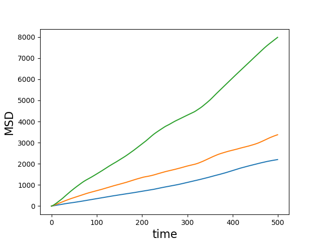
I might as well put a figure here! The lines below will run three simulations, transform the dump files in x,y data files, compute their mean-square displacement using the tidynamics library, and plot the result (with the attached file plot_example_msd.py.

$ parallel run_one ::: 1 2 3
$ for i in 1 2 3 ; do grep '^1 ' langevin_${i}.dump | awk '{print $2 " " $3}' > lxy_${i}.txt ; done
$ for i in 1 2 3 ; do python3 ~/code/tidynamics/examples/tidynamics_tool.py msd lxy_${i}.txt lmsd_${i}.txt; done
$ python3 plot_example_msd.py --dt 1.0 --data lmsd_{1..3}.txt

Remarks

1. This approach allows to have a postprocessing step run directly after the simulation in the same "slot".
2. Several seeds can be passed, which is useful for LAMMPS.
3. This method is useful for simulations with a low count of particles. Parallel computation (as in using MPI, not the GNU Parallel program) involves unnecessary overhead for such simulations.
4. If there is one (or a few) long-running simulation, you might end up with a single running process. The method here is suited for many small runs of similar duration.

Comments welcome via twitter, in the disqus thread below, or by email (pdebuyl at domainname of this blog).